If you regularly work with Excel spreadsheets, you probably find yourself repeating the same steps over and over. Wouldn’t it be nice to click a button and have those tasks happen automatically?
That’s where Excel macros come in. You can use macros to automate repetitive tasks, which can save you a lot of time and effort.
What is an Excel macro?
An Excel macro is a recorded sequence of Excel commands and actions that you can play back as many times as you want. Macros can be used to automate just about any sequence of tasks in Excel, from something as simple as entering your company’s name and address into a spreadsheet to something as complex as creating a custom report. If you can do it in Excel, you can probably automate it with a macro.
To use a macro, you first need to record it. You perform the sequence of steps you want to automate, and Excel tracks them all and saves them in the macro. Once you’ve recorded a macro, you can run it again at any time. You can even assign a keyboard shortcut to a macro, so you can run it with just a few keystrokes.
Excel macros are based on Microsoft’s Visual Basic for Applications (VBA) programming language. When you record a macro, Excel translates your actions into VBA code under the hood. So in addition to creating macros by recording them, you can also write them manually in VBA code. In this article, I will focus primarily on creating macros by recording them — the simplest and quickest method. After that, I will discuss how you can edit or write macros from scratch using VBA and provide some resources for self-learning.
How to record a macro
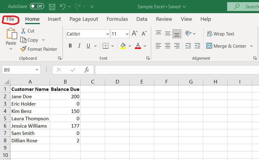
To help illustrate this process, I will use a small sample data set. Let’s suppose that we are responsible for taking customer names and balances and performing two tasks: first splitting the customer’s name into separate first and last names, and then highlighting everyone who has a balance due that is greater than zero. In this example, we have been given seven customers to work with.
 Shimon Brathwaite/IDG
Our starting data set. Note the File menu at the left end of the Excel Ribbon. (Click image to enlarge it.)
To create a macro, we’ll use the Developer tab in the Ribbon toolbar at the top of the Excel window. This is not present by default, so we will need to add it. Click on the File tab at the far left of the Ribbon (highlighted in the screenshot above) and then, on the screen that appears, click Options at the bottom of the left column.
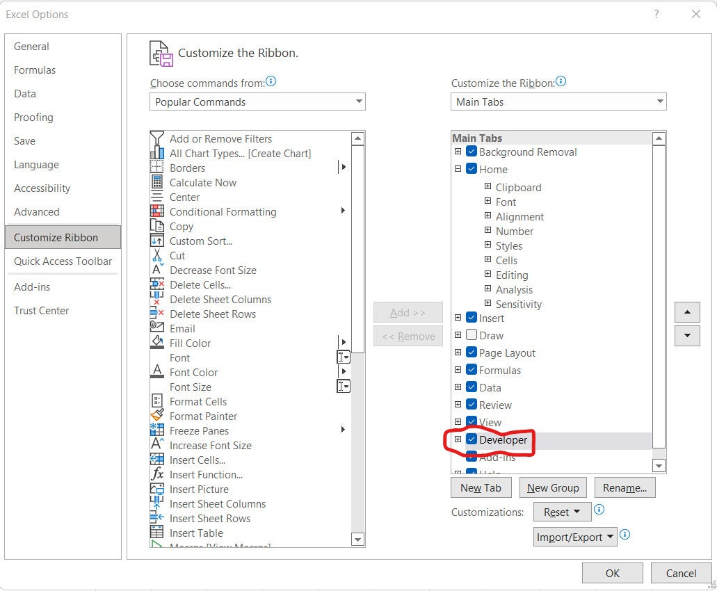
The Excel Options screen appears. Select Customize Ribbon from the left navigation bar. Then, in the “Customize the Ribbon” area on the right, look in the “Main Tabs” list and check the Developer checkbox. Click OK.
 Shimon Brathwaite/IDG
Check the Developer checkbox to turn on the Developer tab in the Ribbon. (Click image to enlarge it.)
(In macOS, click the Excel menu at the top of the screen and choose Preferences > Ribbon & Toolbar. In the “Customize the Ribbon” area on the right, look in the “Main Tabs” list and check the Developer checkbox. Click Save.)
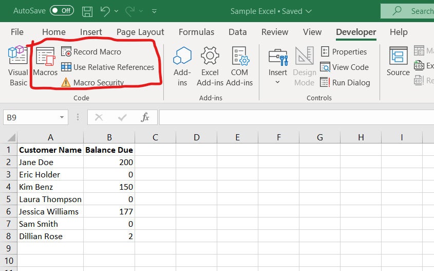
Once you have the Developer tab, click on it and you will see options similar to those shown on the screen below.
 Shimon Brathwaite/IDG
The highlighted commands on the Developer tab help you record and manage macros. (Click image to enlarge it.)
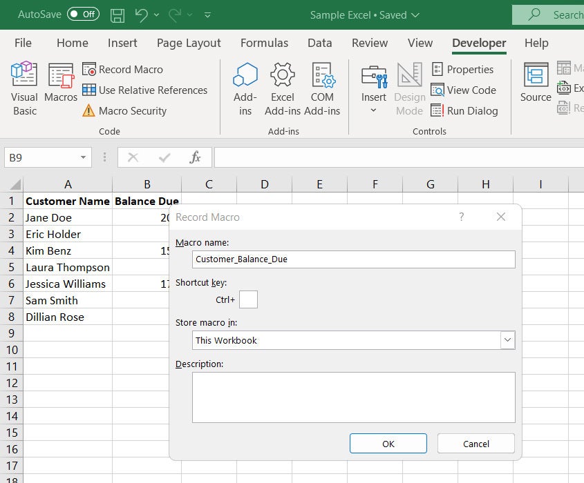
To start recording your first macro, click on the Record Macro button, and you will be presented with the options below. First, create a name for your macro, keeping in mind that you can’t use spaces. For readability, you may want to separate words with something like _ or -. Then add a shortcut key or description if you like, but these are not required.
 Shimon Brathwaite/IDG
To get started, give your macro a name. (Click image to enlarge it.)
Once you hit OK, the icon should change to indicate that the macro is recording your actions. It’s important that you only perform the actions that you want the macro to do and nothing else from this point until you click on Stop Recording.
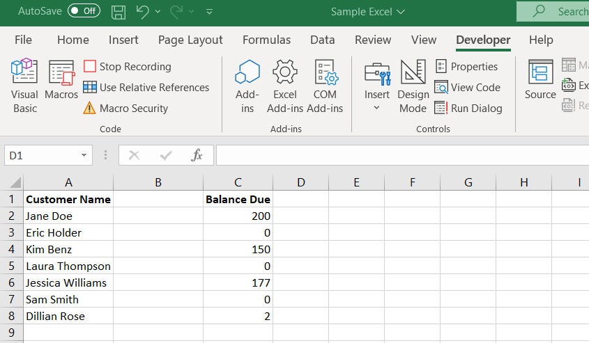
Now that the macro is recording, let’s begin our tasks. First, highlight the Balance Due column, then right-click and select Insert Column. This will add a new column in between the Customer Name and Balance Due columns.
 Shimon Brathwaite/IDG
Insert a new column to the left of the Balance Due column. (Click image to enlarge it.)
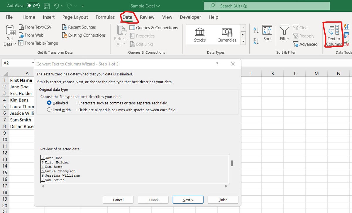
Next, we’ll rename the columns, replacing “Customer Name” with “First Name” and adding the heading “Last Name” to the column we just created. Select the customer names in the first column (cells A:2 to A:8), select the Data tab in the Ribbon, and select the Text to Columns command.
A wizard appears showing the following options. Select Delimited and hit Next.
 Shimon Brathwaite/IDG
On the first screen of the Convert Text to Columns Wizard, select Delimited. (Click image to enlarge it.)
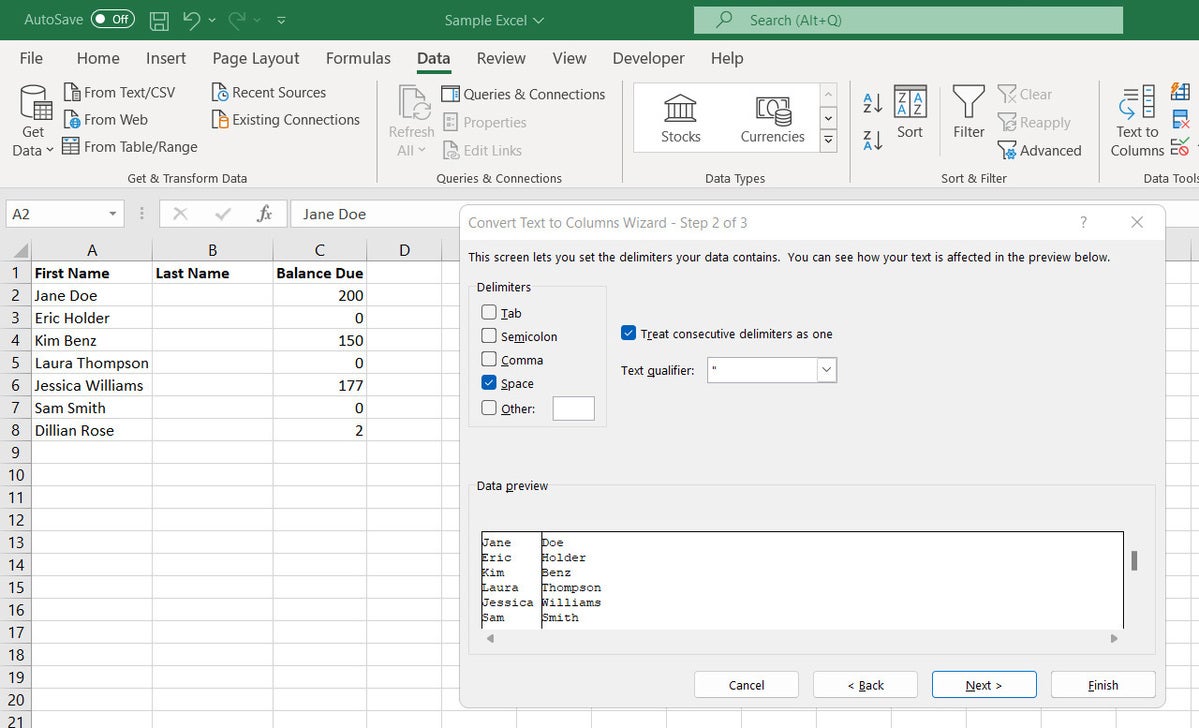
Next, select the Space checkbox to designate that words separated by a space should go into separate columns. Click Next.
 Shimon Brathwaite/IDG
On screen 2 of the wizard, select Space as your delimiter. (Click image to enlarge it.)
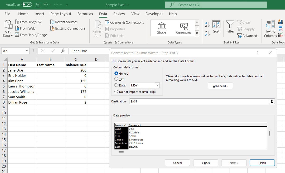
For the last option, keep everything the same and hit Finish.
 Shimon Brathwaite/IDG
Don’t make any changes to the last screen of the wizard. (Click image to enlarge it.)
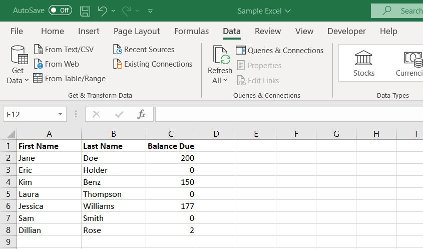
You should have the following result, with first and last names in separate columns.
 Shimon Brathwaite/IDG
The first and last names are now in separate columns. (Click image to enlarge it.)
Lastly, we need to highlight every customer with a balance of more than zero. Highlight all of the data in the third column (cells C:2 to C:8) and then click Home > Conditional Formatting.
 Shimon Brathwaite/IDG
The final step is to apply conditional formatting rules to the data. (Click image to enlarge it.)
Choose Highlight Cell Rules and then Greater Than. Enter 0 and click OK to highlight every customer who has a balance greater than zero.
 Shimon Brathwaite/IDG
Formatting cells that are greater than zero.
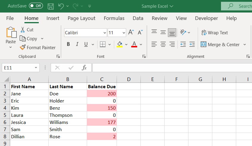
This should be the final result:
 Shimon Brathwaite/IDG
All cells with a balance of greater than zero are now highlighted in light red. (Click image to enlarge it.)
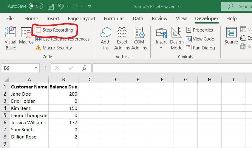
Now that you have completed the tasks sequence, go back to the Developer tab and click Stop Recording. Your first Excel macro is complete.
 Shimon Brathwaite/IDG
When you’re done recording your macro, hit Stop Recording. (Click image to enlarge it.)
Important notes about working with macros
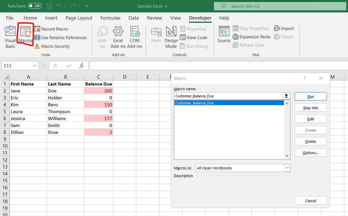
If you want to run your macro again, simply click on the Macros button and it will be available for you to run. Or, if you assigned the macro a shortcut, simply press the key combination to run it.
 Shimon Brathwaite/IDG
Click the Macros button at any time to see the list of macros available for the workbook. (Click image to enlarge it.)
Note that you cannot save a spreadsheet with macros as a traditional .xlsx workbook. You must save it as an Excel Macro-Enabled Workbook (.xlsm) to avoid losing your macros.
 Shimon Brathwaite/IDG
Save your workbook in .xlsm format to preserve its macros. (Click image to enlarge it.)
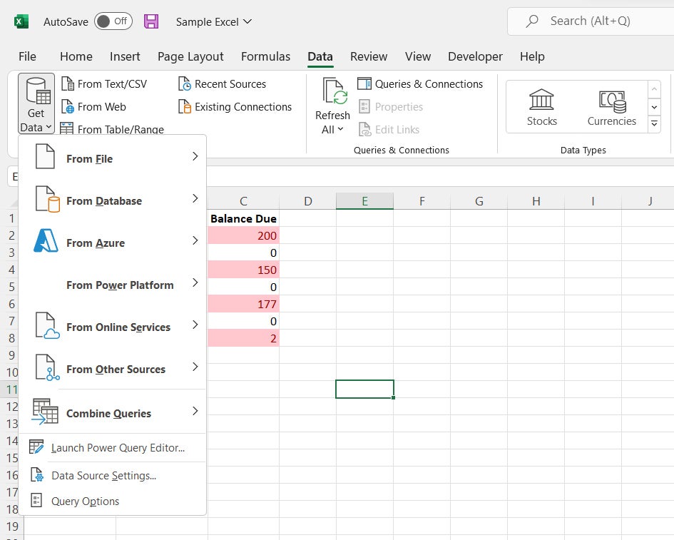
Once you’ve made that change, any time you want to work with a fresh data set you can simply reopen the workbook and import the data you want to work on by going to the Data tab and selecting Get Data. You will be able to import data from files, databases, and other online services.
 Shimon Brathwaite/IDG
Save your workbook in .xlsm format to preserve its macros. (Click image to enlarge it.)
Be aware that in many cases macros are disabled by default. That’s because, as Microsoft notes, “VBA macros are a common way for malicious actors to gain access to deploy malware and ransomware.” To protect organizations from such threats, Microsoft now blocks macros in files from the internet — and sometimes in those stored on the company’s shared drives. Your organization may have imposed additional restrictions on macros.
So whenever you open an Excel workbook with macros in it (including your own), there is a chance that you will see a warning message like the one below. If your workbook is one that you created or from a trusted source, go ahead and enable it. If the macro is from an untrusted source, however, don’t enable it, because it may be malware.
 Shimon Brathwaite/IDG
You might see a warning when you open a workbook with macros in it.
Another important feature to be aware of when recording macros is the use of relative references. This feature makes it so that regardless of where the data begins on the spreadsheet, the macro will be able to find it and start the processing there.
For example, the macro we created will always begin processing at column A because relative references were not toggled on. However, if we did the same operations but clicked on Use Relative References first, then the macro would be able to detect where the information starts (Column C, for instance) and begin its processing from that point. This feature is useful if the data you are working with will not always start at the same point.
 Shimon Brathwaite/IDG
Select Use Relative References if your data won’t always start at the same point in the worksheet.
How to edit or create a macro with code
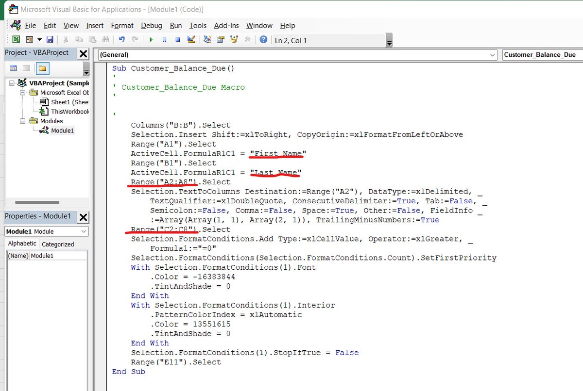
If you want to see the VBA code behind a macro, go to the Developer tab, click Macro, select the macro, and then click Edit.
You will be taken to a pane where you can see the source code for the macro you created. In the screenshot below, the underlined items show actions that we performed, such as changing the names of the headings and selecting rows. You can alter these for different use cases. For example, if the data you work with runs from range A1:A20, you may want to expand the range to include all possible cells.
 Shimon Brathwaite/IDG
Peeking at the code that underlies a macro. (Click image to enlarge it.)
If want to try your hand at writing macros from scratch, there are several resources online for learning to write VBA scripts, including Codewars, Udemy, and Codecademy. Back in Excel, click Developer > Macros > Create. You’ll be taken to a blank pane where you can write VBA code.


