Data comes in from an increasing number of sources these days. For decades, data stores were primarily built by good old data entry. But today we cull data from a range of sources including IoT devices, social media feeds, email, and other sources outside of traditional database platforms. That means the data isn’t always free of errors, blank spaces, or junk characters, and it may be inconsistently formatted from source to source.
If you work with data, at some point you will have the unenviable task of cleaning it. Data cleaning, or cleansing, is a method to get rid of syntax errors, typographical errors, and broken or fragmented records; remove duplicate records; and/or reformat data so it’s easier to work with. It’s also a means to extract specific bits of data from a larger set.
The good news is you have a tool at your disposal for automating much of the process, and that is Microsoft Excel. One obvious way to clean up data in Excel is to use the Find and Replace function, but Excel does a whole lot more.
Excel 2016 and later include a powerful set of tools for sourcing and managing data called Get & Transform. (These tools are also available for Excel 2010 and 2013 as a downloadable add-in called Power Query.) If you’re serious about importing and working with data, it’s well worth your time to investigate Get & Transform/Power Query.
But many business users don’t need such advanced features. If you’re looking for a few quick tricks to clean up your spreadsheets, keep reading. Using a few simple commands, you can eliminate blank cells, merge or split columns, deduplicate data, and more in no time.
1. Deduplicate your data with the EXACT and COUNTIF commands
There are multiple ways to remove duplicates in Excel. Let’s start with the most basic. In Excel 2010 and later, under the Data tab is an option labeled Remove Duplicates. Select the entire data set with Ctrl-A or a partial range with a click and drag. Then go to the Data tab, and in the Data Tools group, select Remove Duplicates. If your data has headers, make sure the “My data has headers” option is checked in the dialog box that pops up, and then click OK.
Remove Duplicates does just what it says: Once you click OK, the duplicates are gone. If you want more flexibility, there are other options to flag duplicates so you can decide what further action to take.
The first is the EXACT command. It compares any two columns and returns TRUE for an exact match or FALSE for no match. The syntax is:
=EXACT(first_cell,second_cell)
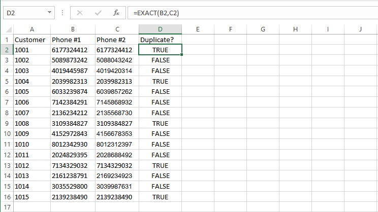
So in comparing a sheet with two columns of phone numbers, with the phone numbers in columns B and C, in cell D2, enter:
=EXACT(B2,C2)
When you press Enter, a value of TRUE or FALSE will appear in cell D2. Now you need to duplicate the formula for the rest of the rows in the data set. Copy cell D2, select all of the cells below it to the bottom of the data set, and hit Enter. Your formula will be duplicated all the way down, always returning results from the data in its own row. You can then sort the rows by which are true and false and act accordingly.
 IDG
IDG
Flagging duplicated data with EXACT. (Click image to enlarge it.)
If you have a large data set, there’s an even better shortcut for pasting the formula down the column: With the cell containing the formula selected, hover your cursor over the lower right corner until you see the cursor change into a thin plus sign. Double-click, and the formula will fill in the rest of the column.
EXACT is great for comparing cells within the same row. The COUNTIF function is great for comparing cells within the same column. It is used for counting cells within a specified range that meet a certain criteria or condition. COUNTIF uses the following syntax:
COUNTIF(range, criteria)
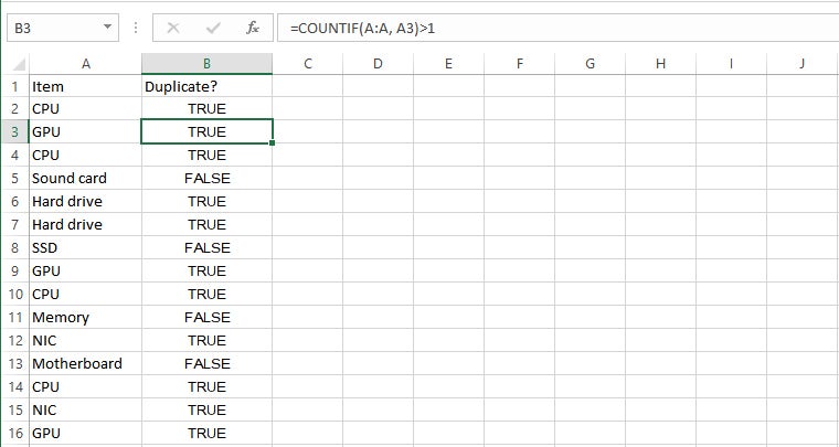
Range is straightforward: it is the number of rows to count, like A2:A100 to check 99 rows. Criteria can be almost anything. Say you want to determine if the same entry can be found in a column of data. Entering =COUNTIF(A:A, A2)>1 in cell B2 will tell if the entry in cell A2 is duplicated after the first instance. Then copy the formula and paste it into the rows you want to check.
 IDG
IDG
Flagging duplicated data with COUNTIF. (Click image to enlarge it.)
FALSE is found only in the rows where there is a single entry. TRUE is returned for the many CPUs, GPUs, hard drives, and NICs, but FALSE shows for sound card, SSD, memory and motherboard because there is only one entry for each.
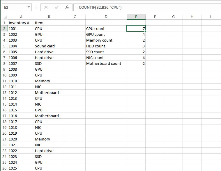
You can also use COUNTIF do a count of items in a column. Using a similar list of components as above, we counted the number of times each component appeared by entering =COUNTIF(B2:B26, "CPU") in cell E2, then changing the formula in each row down column E to look for the different component names.
 IDG
IDG
Using COUNTIF to count the number of various items in a column. (Click image to enlarge it.)
Now you know the number of times each word or phrase, in this case computer components, appeared in the column. From there you can take whatever steps you deem appropriate.
2. Clear out extra spaces with TRIM
The TRIM command is a major cleaning function. It helps you to find and remove junk characters, most notably extra spaces, leaving only a single space between words and no space at the start or end of the text.
The syntax is quite simple:
=TRIM(cell)
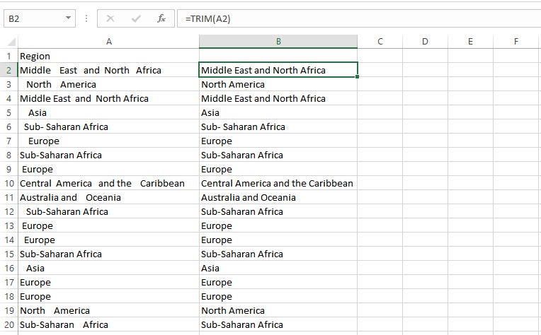
Enter the =TRIM command in the column next to the one you want to clean. So to clean column A, in cell B2 enter =TRIM(A2) for the first cell under the header. Then copy and paste the B2 formula down the column to process all of the other rows of messy data.
 IDG
IDG
Eliminating blank spaces with TRIM. (Click image to enlarge it.)
If in addition to extra spaces your data contains line breaks and non-printing characters, use =TRIM(CLEAN(A2)) to delete the first 32 non-printing characters in the in the 7-bit ASCII code system.
TRIM has its limitations. TRIM is useful when cleaning up text that has come from other applications or environments, because it only removes the ASCII space character, but note that it cannot remove non-breaking spaces used in web pages.
3. Replace junk characters with SUBSTITUTE
Find and replace isn’t the most elegant of replacement tools, because it can only do one character or word at a time. A faster way to do multiple characters at once is to use the SUBSTITUTE function. The syntax is as follows:
=SUBSTITUTE(cell, old_text, new_text, instance_num)
All these elements straightforward: “cell” is the cell that contains the string you want replaced; “old_text” is the sequence of characters that you want to replace; “new_text” is what to insert; and “instance_num,” which is optional, tells Excel how many times it should replace “old_text” if it finds more than one instance.
So let’s say you have goofed up cells that list the year as 2018 and want to replace all of the 2018s with 2019. Use:
=SUBSTITUTE(A2, "2018", "2019")
Then copy and paste the formula down all of the rows to make the replacement. A few more examples:
- =SUBSTITUTE(A1,"A","C") replaces A's with C's
- =SUBSTITUTE(A1,"A","a") replaces uppercase A’s with lowercase a’s
- =SUBSTITUTE(A1,"A","Z",1) replaces the first A in the cell with Z
- =SUBSTITUTE(A1,"#","") replaces # with nothing
Those are pretty simple and can be done with the regular find and replace. But SUBSTITUTE does much more. In the following example, we clean up and reformat telephone numbers to strip out all extraneous characters, then use Excel's formatting to convert the numbers into proper format. Phone numbers can be fouled up on data entry in a variety of ways. SUBSTITUTE lets you cover all the bases at once.
The formula below uses a series of nested SUBSTITUTE functions to strip out open and close parentheses, hyphens, spaces, and periods in cell B2:
=SUBSTITUTE(SUBSTITUTE(SUBSTITUTE(SUBSTITUTE(SUBSTITUTE(B2,"(",""),")",""),"-","")," ",""),".","")
The formula runs from the inside out, with each SUBSTITUTE removing one character, and each character in quotes. The innermost SUBSTITUTE (just before the “B2”) removes the left parenthesis symbol — i.e., it replaces the symbol with nothing:
SUBSTITUTE(B2,"(","")
The next SUBSTITUTE out removes the right parenthesis symbol, the next one out after that removes the hyphen, and so on. This can get confusing, because each SUBSTITUTE requires the text to be replaced in quotes (“old_text”), followed by the empty set of quotes (“new_text,” which in this case is nothing), followed by a closing parenthesis — and all these elements are separated by commas. You can add as many SUBSTITUTEs to remove as many characters as you want.
 IDG
IDG
Nested SUBSTITUTE commands clear out parentheses, hyphens, and spaces simultaneously for the results in column C. (Click image to enlarge it.)
Pasting the formula down the column results in a column of cleaned, unformatted numbers — column C in the screenshot above. To get them formatted as in column D, copy all the cleaned numbers and paste them into the Formatted column. With the numbers in column D still selected, find the Number section in the middle of the Ribbon’s Home tab and click the drop-down list showing “General.” Select More Number Formats from the bottom of the list. In the dialog box that appears, select Special from the Category list on the left, select Phone Number from the Type list in the center, and click OK.
4. Edit capitalization with PROPER, UPPER, and LOWER
Text can be changed to all caps, no caps, or proper case (a.k.a. title case) the same way TRIM lets you remove spaces. This has to be done one column at a time and does not work on rows.
First, create a new column, preferably next to the one you are cleaning. Let’s say data entries start at cell A2. In B2, enter =UPPER(A2), =LOWER(A2) or =PROPER(A2) and hit Enter. In B2, the data from A2 will be changed to the form you chose. Then copy the formula down the rest of the column. You can see the results for all three commands in the screenshot below.
 IDG
IDG
Country names formatted with the PROPER, UPPER, and LOWER commands. (Click image to enlarge it.)
5. Merge or split columns
Let’s say you want to merge columns A and B into one. You might want to merge first and last name together into one cell, or perhaps cities with two names (e.g., New York) got split into two cells and you want them in one cell.
In a new column, place your cursor in cell C2 (assuming you have a header in row 1) and type:
=A2&" "&B2
The quotation marks are to put a space between the two cell entries. If you don’t want a space, then it’s simply:
=A2&B2
Then copy the formula down the rest of the column.
The reverse of merging cells is splitting text inside one column into two or more columns. For instance, your data might include first and last names of customers in a single column, but you need to separate them so that you can sort them alphabetically by last name. When data is obtained from a non-structured source, like a text file, you might even find an entire line of data entries crammed in one cell.
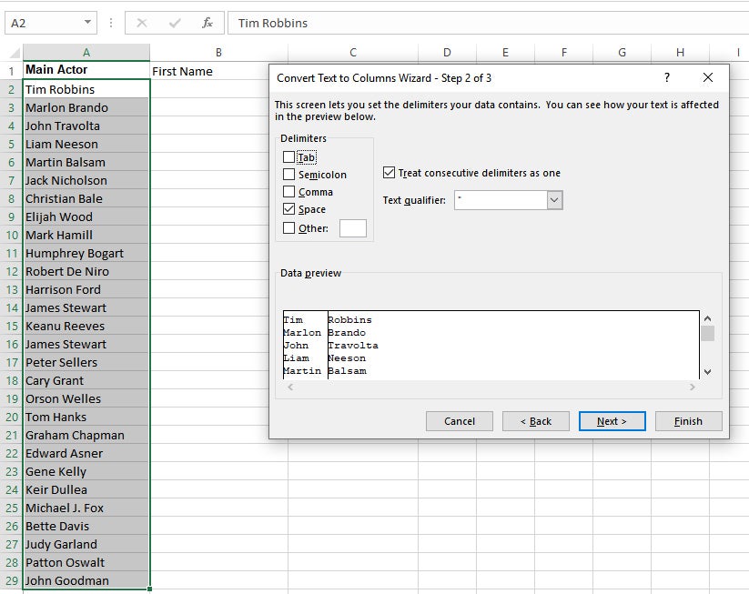
You can split this text into multiple cells by using Text to Columns function. We’ll demonstrate with the first and last names example. Select the cells you want to parse, then go to the Data tab on the Ribbon and in the Data Tools section, click Text to Columns. This opens the Convert Text to Columns Wizard.
On the first screen, the wizard determines that data is delimited — i.e., the items in each cell are separated by spaces, commas, and/or other characters. Choose Delimited if it is not already selected and click Next. On the next screen you can select one or more delimiters to have the wizard look for. Your options are Tab, Semicolon, Space, Comma, or Other, where you can enter an oddball character such as a pipe (|). Check the appropriate box(es). A preview box below shows how the data will be split.
 IDG
IDG
Splitting cells using the Convert Text to Columns Wizard. (Click image to enlarge it.)
Click Next, and the Column data format screen will come up, allowing you to select the data format for the new columns or go with the default, which is that the new columns will have the same format as the original cell. Click Finish, and text in the original column will now appear in two columns.
 IDG
IDG
The first and last names from column A now appear split in columns B and C, with a couple of errors that need to be fixed manually. (Click image to enlarge it.)
As the second image shows, it’s not foolproof: Robert De Niro and Michael J. Fox got split an extra time. But two minor fixes are easy to make considering the time saved splitting out the first and last names.
6. Find and replace blank cells
Blank cells can mess with analytics if not treated beforehand. Cells should at least have 0, null, or Not Available entries. There is a way you can select all the blank cells at once in Excel.
- Select the entire data set.
- Press F5. The Go To dialog box appears.
- Click on the Special… button to open the Go To Special dialog box.
- Select the Blanks radio button and click OK.
This selects all the blank cells in your data set. If you want to enter 0, null, or Not Available in all the empty cells at once, just type it and press Ctrl + Enter.
7. Extract partial values from a column
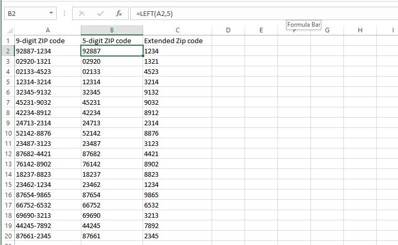
You can extract partial values from a cell from the left, right, or middle using the LEFT, RIGHT, and MID commands. The syntax for the first two is =LEFT(cell,length) and =RIGHT(cell,length). Say you have a column with 9-digit ZIP codes and you’d like to separate things out, so the main five digits are in one column and the extended ZIP is in a second column.
If your ZIP code list starts in cell A2, in the cell next to it (B2), enter:
=LEFT(A2,5)
In the next column over, use:
=RIGHT(A2,4)
As always, copy the formula in the first cell of each column down the column. And voila! You have split out your ZIP codes.
 IDG
IDG
Using LEFT and RIGHT to split 9-digit ZIP codes. (Click image to enlarge it.)
MID is a little more complex; it requires one more digit:
=MID(cell,startnum,length)
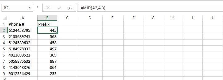
Let’s say you have cells with complete phone numbers but want only the prefix — the first three digits after the area code. Again assuming the data starts in cell A2, you would use =MID(A2,4,3) in cell B2. This tells Excel to count to the fourth digit in the cell and extract three digits. Once again, copy the formula in the first cell down the column. From there you can sort by phone number prefix, something done in targeted marketing.
 IDG
IDG
Extracting phone number prefixes with MID. (Click image to enlarge it.)
8. Unpivot your data
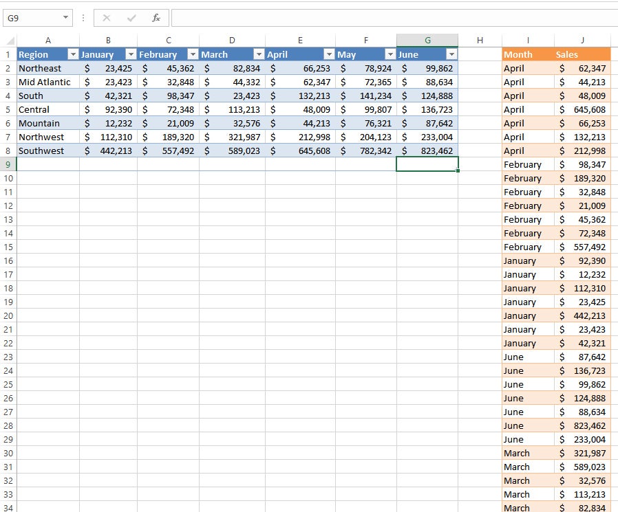
Horizontal columns with aggregate data (a.k.a. crosstab format) don’t lend themselves well to being converted to a PivotTable; vertical rows with separate data points (a.k.a. tabular format) do. The Unpivot command takes a data set that stretches horizontally across the top of the report and makes a new chart where the original horizontal columns are separated into individual data points in vertical rows, which is the best way for further analysis with PivotTables.
Unpivot is one of the tools in the Get & Transform/Power Query toolbox. It’s built into Excel 2016 and later, but to use it in Excel 2010 or 2013, you need to download and install the Power Query add-in.
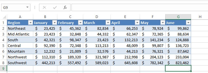
Let’s use a regional sales chart sample, broken down by month. First, make sure the data is in table format, which looks like this:
 IDG
IDG
Before using the Unpivot command, make sure your data is in table format. (Click image to enlarge it.)
If it’s not, put your cursor in any cell in the data set, go to the Insert tab on the Ribbon, click the Table button near the left end of the Ribbon, and click OK. Next, in Excel 2016 and newer, click the Data tab on the Ribbon, and then in the Get & Transform area, click the From Table/Range button to bring up the Power Query Editor window. Select the appropriate columns by clicking the first column you want to unpivot, then holding down the Shift key and clicking the last column. Click the Transform tab in the Power Query window’s Ribbon and select the Unpivot Columns button. Or you can right-click on one of the columns and select Unpivot Columns.
In Excel 2010 or 2013 with Power Query installed, go into the Power Query menu and select From Table/Range; a Power Query window opens. Select the columns with the figures, not the header information, then the Transform menu item, and click Unpivot Columns — or right-click one of the columns and select Unpivot Columns.
 IDG
IDG
The Power Query Editor window is where you can unpivot your columns. (Click image to enlarge it.)
Your horizontal data is now vertical, ready for PivotTable manipulation. In the Power Query Editor’s Ribbon, go to the Home tab and click the Close & Load button all the way to the left. The tabular version of your data will appear on a new worksheet by default. If you’d rather add it to an existing worksheet (or display it as a PivotTable or PivotChart), instead click the small down arrow in the corner of the Close & Load button, then select the Close & Load To... option from the menu that appears, designate where and how you want the data displayed, and click OK.
 IDG
IDG
The table on the right shows the unpivoted the data from the table on the left. (Click image to enlarge it.)
That’s just one example of what Power Query/Get & Transform can do. It is designed to connect to data sources, then combine and clean that data in one fell swoop through simple wizards. If you’re serious about importing and analyzing data from various sources, Microsoft has some helpful tutorials to get you started with the tools.


