Google Sheets power tips: Create an automatically updating spreadsheet

Tracking basic data in a spreadsheet is pretty simple — it’s remembering to update your data each day, week, or month that can be a problem. But why update manually when you can take advantage of some simple automation tools?

Here’s a step-by-step guide to creating an automatically updating Google Sheet that both scrapes data from the web and automatically updates the spreadsheet. We’ll use “daily local temperature at lunchtime” in this example, but the code can be easily tweaked to fetch and store other data as well.

1. Create a Google Sheets spreadsheet

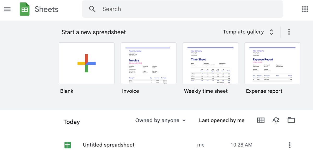
Head to Google Drive or Google Sheets and create a new blank spreadsheet. (If you don’t yet have a Google account, you can sign up there.)

IDG/Sharon Machlis

Title the sheet anything you want, and you’re ready to begin. (The default will be “Untitled spreadsheet,” but you can click on that to change it to something that will better identify it in your list of documents.)

2. Find the “XPath” for the part of the web page you want to scrape

Google Sheets needs an “XPath” selector to pluck just a portion of data from a web page. Fortunately, there’s an easy-to-use point-and-click tool that helps you do just that: SelectorGadget. (There’s a less-than-2-minute video on the site demonstrating how it works.)

Install the SelectorGadget Chrome browser extension, activate it by clicking the browser tool icon, and then click on the section of the page you want to scrape. That section will turn green. The trick is to make sure you’re only selecting that. Other areas of the page may be green or yellow, too. If they are, click on the ones that you want to remove from your selection.

In the image below, I visited the National Weather Service page for Needham, MA, the location of Foundry corporate headquarters. (Foundry is Computerworld’s parent company.)

This page was easy: I clicked the temperature, and it was the only item selected. If others had shown up as green or yellow, I would have clicked those to turn them off in order to make sure my XPath was choosing only what I need.

IDG/Sharon Machlis

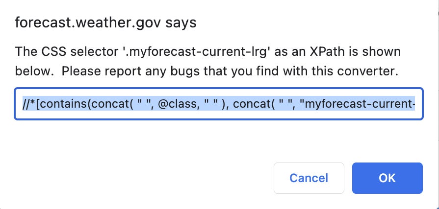
In the bottom right, a selector appears; but that .myforecast-current-lrg is a css selector. I need XPath, which is an option all the way at the bottom right. Click on XPath, and the XPath version will show up looking something like this:

IDG/Sharon Machlis

XPath is often more complicated than CSS, but you don’t need to worry about what all the expressions mean. The one key point is that the XPath selector will end up surrounded by double quotation marks in your Google Sheets formula. Unfortunately, the selector itself also has double quotation marks. That will cause problems, so if your XPath includes double quotation marks, change them all to single quotes manually.

The XPath selector I’ll use in my Google Sheet is now

//*[contains(concat( ' ', @class, ' ' ), concat( ' ', 'myforecast-current-lrg', ' ' ))]  

3. Add your formula

Spreadsheet formulas can do more than math calculations; they can also extract data from web pages. For a Google Sheet, the function to read part of a web page is:

=ImportXML("URL", "XPath selector")

For my National Weather Service Needham, MA page and temperature selector, that’s

=IMPORTXML("https://forecast.weather.gov/MapClick.php?lat=42.2803&lon=-71.2345", "//*[contains(concat( ' ', @class, ' ' ), concat( ' ', 'myforecast-current-lrg', ' ' ))]")

In my spreadsheet’s first column, I’ll list the location I’m tracking. This will make it easy to add additional places to my sheet in the future. I’ll put the formula in the second column.

IDG/Sharon Machlis

And I want the date and time in column C. We’ll take care of that in a moment.

4. Write a function to fetch and store data

The way the spreadsheet is currently set up, the temperature won’t be saved; it will change each time you open the sheet.

To keep historical data as the sheet’s currently designed, I’d need to copy and paste values manually into another cell each time I opened it. That’s not very scalable! Instead, let’s create a new function to 1) Find the first empty row in the sheet and 2) copy the value from cell B2 into another empty cell for storage.

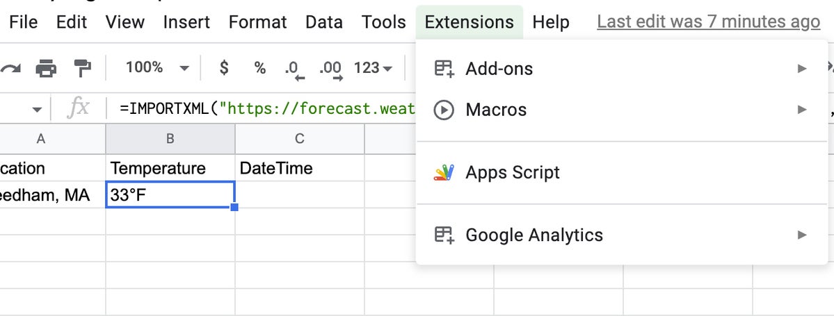
To store data, we’ll need to create a spreadsheet function. Head to Extensions > Apps Script to create functions for the spreadsheet.

IDG/Sharon Machlis

You’ll see a default function pop up called myFunction.

IDG/Sharon Machlis

Change that function name to storeTemperature() (or whatever you might like to call it), and use the following code:

function storeTemperature() {
  var sheet = SpreadsheetApp.getActiveSheet();
  var firstEmptyRow = sheet.getLastRow() + 1;


  // Get current temperature from cell B2
  var currentTempCell = sheet.getRange(2, 2);
  var currentTemp = currentTempCell.getValue();


  // Find first empty cell in column B and add that value
  var newTempCell = sheet.getRange("B" + firstEmptyRow);
  newTempCell.setValue(currentTemp)


  // Get the current date and time add it to same row column C
  var currentDate = Date(); 
  var newDateCell = sheet.getRange("C" + firstEmptyRow);
  newDateCell.setValue(currentDate)


  // Add place name in column A, currently hard coded
  sheet.getRange("A" + firstEmptyRow).setValue("Needham, MA")
}

The first line of code creates a variable for whatever spreadsheet is active, followed by a variable holding the number of that sheet’s first empty row.

In order to read or write data in a Sheets cell, that cell needs to be a range object. Fortunately, it’s easy to turn a spreadsheet’s cell location into a cell range object with yourSheetObject.getRange(). In this example, I called my sheet object sheet (you can call it anything), so the code is sheet.getRange(). getRange takes several formats to identify a cell location, including getRange(3,5) for row 3, column 5, or getRange("B " + 2) for conventional spreadsheet cell syntax like B2.

With that in mind, I can create a variable holding the cell range for cell B2, which is row 2 and column 2, where I know my current temperature sits, using sheet.getRange(2, 2). I then read that value with get.Value() as you can see in the above code.

Next in that code block, I find the first empty row in column B, where I want to add the new temperature, and save that cell as a range object. Then it’s simply a matter of setting that cell’s value with the temperature I just stored.

The final rows do something similar to store the current date and time as well as the hard-coded location.

There are ways to make this code more compact, but I’m sharing a verbose version to make it easier to see what’s going on. In the last line, I tightened it up a bit by combining getRange and setValue in a single line of code, instead of creating a separate variable holding the cell range. Use whichever syntax you prefer.

IDG/Sharon Machlis

Save this by clicking the floppy disk icon above the function code. You’ll probably want to change the default project name to something else. I named mine “Lunchtime Temps.”

You can test your script by clicking the Run button to see what happens in the spreadsheet. If all goes well, you’ll have a new row of data with the current temperature.

5. Schedule your function to auto-run

Last piece: Schedule your function to run automatically. To do this, click on the clock icon on the left to open your script dashboard that shows your current project’s triggers. (There won’t be any yet.) You may be asked to authorize this in your Google account first.

IDG/Sharon Machlis

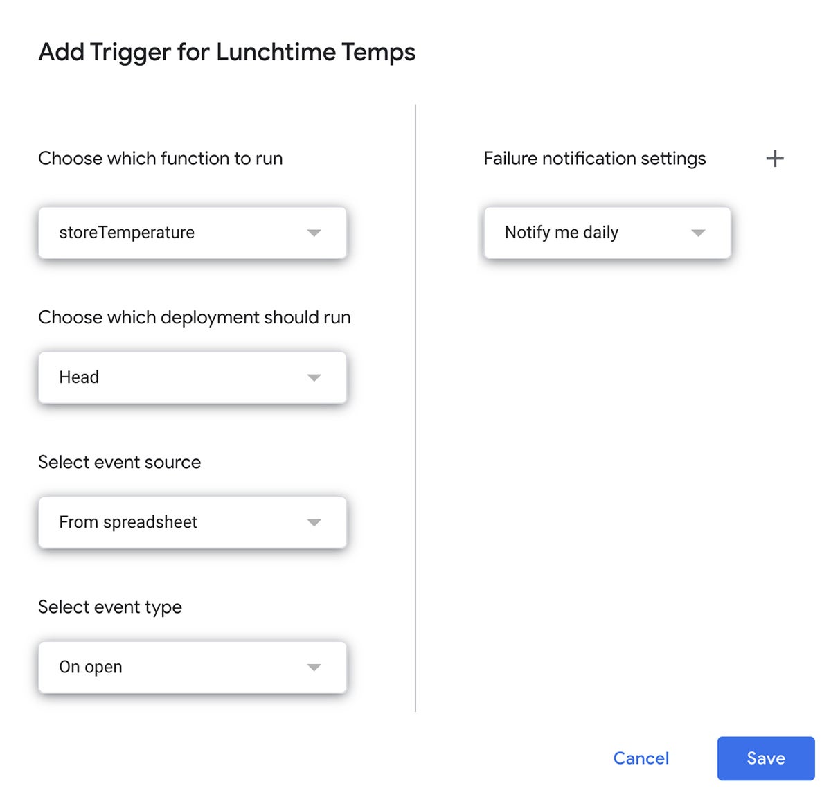
Click on create a new trigger, and a menu pops up.

IDG/Sharon Machlis

If you want your spreadsheet to update on a specific schedule, change the event source from “From spreadsheet” to “Time-driven” and then select whether you want it running hourly, daily, weekly, monthly, or other options.

Then, voila! A self-updating spreadsheet that collects and stores data automatically.

This article was originally published in April 2017 and updated in February 2023.