Have you come to Microsoft Excel 2010 by way of Excel 2007, or did you skip directly from Excel 2003 or an earlier version? Those in the former group are likely to have a very different upgrade experience from those in the latter group.
Share this story: IT folks, we hope you'll pass this guide on to your users to help them learn the Excel 2010 ropes.
If you're in the former group, you'll find a few small interface tweaks and a handful of useful new features in Excel 2010. If you're in the latter group, you'll find an overhauled interface that radically changes how you interact with common features and functions.
Either way, we've got you covered. This cheat sheet shows newcomers to the interface how to get around; it also explores features that are brand-new in Excel 2010. We've noted which sections of the story former Excel 2007 users can skip over.
Get acclimated to the new Excel
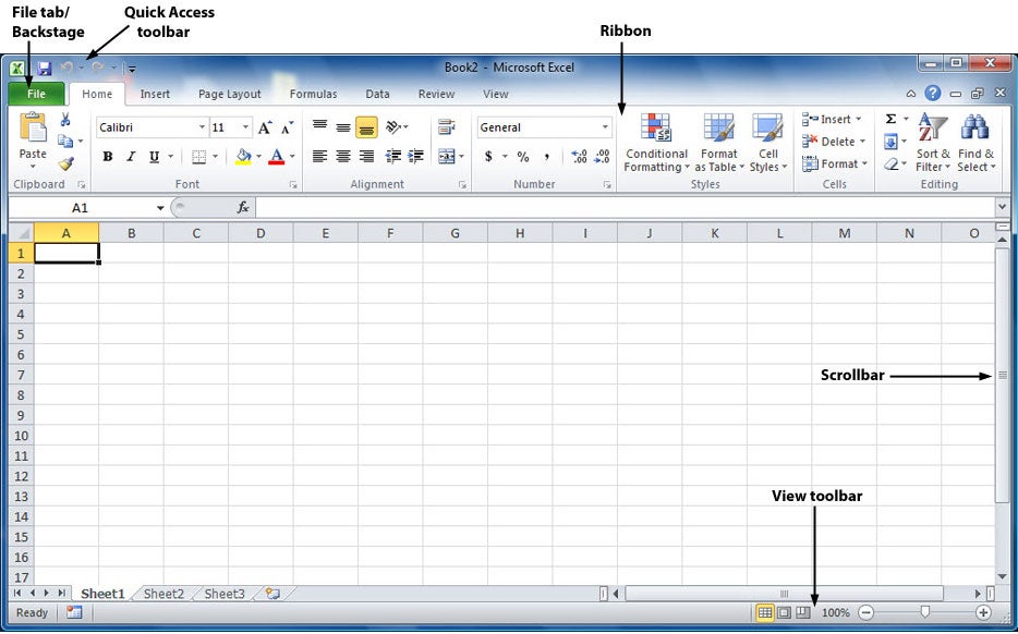
To help you find your way around Excel 2010, here's a quick guided tour of the revamped interface; follow along using the screenshot below.

Get to know Excel 2010's interface. (Click image to enlarge.)
The Quick Access toolbar. Introduced in Excel 2007, this mini-toolbar offers buttons for the most commonly used commands, and you can customize it with whatever buttons you like, as we'll explain later in the story.
The File tab/Backstage. The File tab in Excel 2010 replaces the Office orb button in Excel 2007, which replaced the old File menu found in earlier versions of Excel. Click it, and it leads you to Backstage, a new command center where you can handle an array of tasks, including opening, printing and sharing files; customization; version control and more. As you'll see later in this story, Backstage represents the biggest change in Excel 2010.
The Ribbon. Love it or hate it, the Ribbon is the main way you'll work with Excel. Instead of old-style menus, submenus, sub-submenus and so on, the Ribbon groups small icons for common tasks together in tabs on a big, well, ribbon. So, for example, when you click the Insert tab, the Ribbon appears with buttons for items that you can insert into a spreadsheet, such as charts, tables, PivotTables, clip art or a hyperlink.
The Excel 2010 Ribbon looks and works much the same as the Excel 2007 Ribbon, with one nifty addition: In Excel 2010, you can customize what's on the Ribbon.
The Scrollbar. This is largely unchanged from previous versions of Excel; use it to scroll up and down. At the top, there's a double arrow that, when clicked upon, expands the area at the top of the worksheet that displays the contents of the current cell. Just below the double arrow is a tiny button that looks like a minus sign that lets you split your screen in two.
The View toolbar. As with Excel 2007, there is a View toolbar at the bottom right of the screen that lets you choose between Normal, Page Layout and Page Break Preview -- the latter view shows you how your spreadsheet will look when it prints. There's also a slider that lets you zoom in or out of your document.
Learn to love the Ribbon
If you're comfortable with the Ribbon interface in Excel 2007, you'll be happy to hear that it's basically the same in Excel 2010. You can skip directly to the next section of the story, "Find your way around Backstage," where you'll learn, among other things, how to customize the Ribbon -- a feature that wasn't available in Excel 2007.
If the Ribbon is new to you, here's what you need to know. At first, the Ribbon may be off-putting, but the truth is that once you learn to use it, you'll find that it's far easier to use than the old Excel interface. It does take some getting used to, though.

The default Excel 2010 Ribbon. (Click image to enlarge.)
By default, the Ribbon is divided into eight tabs, with an optional ninth one (Developer). Here's a rundown of the tabs and what each one does:
File (also known as Backstage): As you'll read later in the story, here's where you perform a variety of tasks such as printing, sharing files, customizing the Ribbon and more.
Home: This contains the most commonly used Excel features, such as formatting tables, rows, cells and text; inserting a few basic formulas; and sorting and filtering.
Insert: As the name implies, this tab handles anything you might want to insert into a spreadsheet, such as charts, pictures, clip art, PivotTables, tables, equations, headers and footers. It also lets you insert two new types of content introduced in Excel 2010: Sparklines and Slicers. (More on those later.)
Page Layout: Here's where you change margins, page size and orientation; apply themes; define your print area; set page breaks; specify which rows and columns will print on each page and so on.
Formulas: If you're a spreadsheet jockey, you'll be spending a lot of time on this tab. As the name says, it's where you go to insert and work with formulas. It organizes all of Excel's formulas into categories, such as Financial, Logical, Math & Trig and so on, so they're all within easy reach. And it also gives you quick access to useful formula-checking features, such as error checking and the ability to trace precedents and dependents.
Data: Whatever you need to do with data, you'll do it here. For example, you can use this tab to import data from a wide variety of sources, including the Web, Access, SQL Server, XML import and so on. You can also filter and sort data, validate your data, group and ungroup data, and perform data analysis, among other features.
Review: Need to work in markup mode, review other people's markups or compare documents? This is the tab for you. It also lets you protect worksheets and workbooks, share workbooks, check spelling and grammar, and look up a word in a thesaurus.
View: Here's where to go when you want to change the view in any way, including displaying or turning off gridlines and the formula bar, zooming in and out, splitting and hiding panes, and so on.
Developer: If you write code or create forms and applications for Excel, this is your tab. It also includes macro handling, so power users might also want to visit here every once in a while.
The Developer tab is hidden by default. To display it, click the File tab and choose Options --> Customize Ribbon and then check the box next to Developer in the Customize the Ribbon section.

Get to know how the Ribbon is organized.
Each tab along the Ribbon is organized to make it easy to get your work done. As you can see below, each tab is organized into a series of groups that contain related commands for getting something done -- in our example, handling fonts.
Inside each group is a set of what Microsoft calls command buttons, which carry out commands, display menus and so on. In the example, the featured command button changes the font size.
There's also a small diagonal arrow in the bottom-right corner of some groups, which Microsoft calls a dialog box launcher. Click it to display more options related to the group.
All that seems simple enough...so it's time to throw a curveball at you. The Ribbon is context-sensitive, changing according to what you're doing. Depending on the task you're engaged in, it sometimes adds more tabs and subtabs.
For example, when you insert and highlight a chart, several entirely new tabs appear: Design, Layout and Format, with a Chart Tools supertitle on top, as you can see here.

The Chart Tools tab appears when you need it.
Other "now you see them, now you don't" tabs include Picture Tools, Table Tools and SmartArt Tools -- all of which appear in response to various actions you take in Excel.
Find your way around Backstage
Backstage is a one-stop shop for doing common tasks such as saving, printing and sharing files, getting information about your spreadsheets, and more. It brings together a variety of functions that were found in multiple locations in previous versions of Excel.
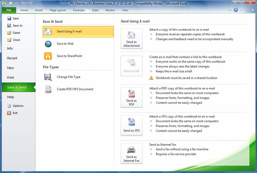
When you click the File tab on the Ribbon, you're sent to Backstage. The Ribbon disappears and is replaced by a series of items down the left-hand side of the screen, most of which are self-explanatory, such as Save, Save As, Open, Close, Recent, New, Print and Help.

Backstage in Excel 2010 is a one-stop shop for performing a wide variety of tasks. (Click image to enlarge.)
However, there are three choices that are not so self-explanatory but can be enormously helpful:
Info
On the far right of the screen, Info shows useful information about the file you're working on, including its size, title, author, and tags, as well as the last time it was modified and printed, the last person who modified it, and similar information.
But finding information about the file is just the start of what you can do when you click the Info button. If you've opened a document that's not in the latest Excel format (.xlsx), such as a .xls file, you'll see a Compatibility Mode area, which lets you know that some of the newest Excel features have been disabled to ensure compatibility with the older format. Click the Convert button if you want to convert the file into the new format, but note that some layout formatting may change.
Click Protect Workbook in the Permissions area to specify who has rights to read and edit the file. You can also restrict all editing or set similar permissions options.
Before sharing the file with anyone, click Check for Issues in the Prepare for Sharing area -- this will let you see if you've left any hidden information or fields in the document, for instance, or if the file is incompatible with earlier versions of Excel.
Click Manage Versions in the Versions area if you would like to see earlier versions of the file that have been auto-saved.
Save & Send
Excel 2010 was built for a world in which documents and their contents are meant to be shared in many ways, such as via email, in Microsoft's SharePoint collaboration software, or in the cloud. Click Save & Send, and you get options to do all that and more.

The Save & Send option in Backstage offers several ways to share your documents with others. (Click image to enlarge.)
Send Using E-mail attaches the current document to a blank outgoing email, using your default mail program. You can send it in its current format, as a PDF or an XPS (a PDF-like Microsoft format) file, or as an Internet fax. If the file is stored in a shared location, you can choose to email a link rather than an attachment.
Save to Web lets you save the file to Windows Live SkyDrive, Microsoft's cloud-based file storage site. Of course, you need to have a SkyDrive account, and you'll be prompted to log in the first time you use this feature. After that, you can save the current file to any of your folders on SkyDrive.
Save to SharePoint lets you save your file to a SharePoint server for sharing with co-workers -- check with your IT department if you don't have your organization's SharePoint access information.
The Save & Send section of Backstage also lets you convert the file to a variety of other file types, such as tab-delimited text, comma-delimited text (.csv), OpenDocument Spreadsheet (.ods), XML, PDF, XPS and many others. Note that if you do this, you may lose some layout formatting.
Options
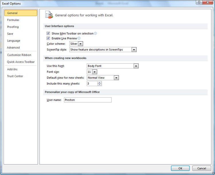
Here's where you can customize the way Excel looks and works, taking care of everything from how text and formatting marks display, to what buttons appear in the Quick Access toolbar, to proofing options and more.
New to Excel 2010 is the ability to customize the Ribbon. After you click Options, click Customize Ribbon, and you can choose what you want shown on each of the Ribbon's tabs.

The Options screen, accessed via Backstage, is where you can customize the way Excel 2010 looks and feels to your heart's content. (Click image to enlarge.)
Show trends with Sparklines
Though creating charts and graphs in Excel has become easier over the years, such visualizations are often overkill. They take up space, and sometimes you spend more time getting the look right than you should.
New in Excel 2010, Sparklines are smart, simple graphics you add to a single cell to give quick visual representations of data, especially data that changes over time -- for example, unit sales of a particular item over the course of several years. A Sparkline can show you at a glance the historic ups and downs of that item.
Sparklines come in three flavors: line, column and win/loss. As with any Excel chart, the Sparkline is redrawn automatically when you change the data in its data range.
To create a Sparkline, move your cursor to the cell where you want to insert the mini-chart. On the Insert tab, find the Sparklines group in the middle of the Ribbon. Click on the type of Sparkline (line, column, win/loss) you want. In the pop-up dialog box, choose the source range (the data you want to plot) and click OK.

Sparklines are cell-sized charts that can show trends at a glance. (Click image to enlarge.)
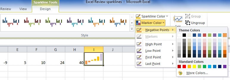
Notice that the Ribbon changes to display the Sparkline Tools/Design tab, where you can modify the properties of the graphic -- switching among the three types of Sparklines, changing the overall color scheme or adding color to individual elements. Negative values can be displayed as red dots (in line Sparklines) or red columns (in column and win/loss Sparklines).

Sparklines can be customized in several ways. This win/loss Sparkline has been enlarged by increasing the row height. (Click image to enlarge.)


